1. The Paradigm Shift: Why Geometry Outpaced Mechanics
For nearly three centuries, the production of precision optics was governed by the Principle of Kinematic Averaging. This classical approach, perfected during the telescope-making eras of Newton and Herschel, relied on the “Self-Correction” that occurs when two rigid surfaces—the tool (lap) and the workpiece—are rubbed together with a loose abrasive slurry. Through random, high-frequency motion, the high spots on both surfaces are worn down more rapidly than the low spots, naturally converging toward a perfect sphere. In this paradigm, precision was a byproduct of time and mechanical probability.
The Convergence Crisis in the Aspheric Era
The shift from spherical optics to Aspheric and Freeform geometries destroyed this traditional harmony. An aspheric surface has no single center of curvature; its slope changes continuously across the radial profile. When a traditional rigid lap attempts to polish an asphere, it encounters a “Geometric Mismatch.” The tool cannot conform to the varying curvature, leading to localized pressure spikes. This results in the catastrophic failure known as Edge Roll-off and the creation of mid-spatial frequency ripples that scatter light and degrade the optical wavefront.
As optical requirements moved from the micron level to the nanometer and eventually the picometer level (for EUV lithography), we reached the Mechanical Stalemate. No matter how stiff the machine bed or how accurate the air-bearing spindle, mechanical components are subject to infinitesimal vibrations and thermal fluctuations. In a purely mechanical process, the “Noise” of the machine is eventually engraved into the glass. The industry realized a fundamental hard truth: Mechanics alone can no longer provide the necessary fidelity; the solution must be mathematical.
Enter Determinism: The Software-Driven Surface
Magnetorheological Finishing (MRF) represents the Deterministic Revolution. It abandons the idea of “averaging” entirely. Instead of hoping the surface converges through random motion, MRF treats material removal as a discrete, calculated subtraction. By replacing the rigid tool with a compliant, magnetically-controlled fluid ribbon, the process decouples the tool’s shape from the lens’s shape. This allows for a Sub-Aperture approach where the machine executes a “Correction Function” derived from metrology data.
In this new paradigm, the “Iron” of the machine (its spindles and guideways) provides the foundation, but the “Fluid” and the “Software” provide the precision. We have moved from a world of mechanical probability to a world of Mathematical Inverse Modeling. This report serves as the final chapter in our exploration of ultra-precision manufacturing, demonstrating how MRF acts as the ultimate “Inverse Problem Solver,” converting mechanical error into optical perfection.
The Paradigm Axiom: “Traditional polishing smooths surfaces through hope and probability. MRF corrects geometry through calculation and determinism. In the nanometer era, we do not polish lenses; we solve them.”
2. The Fluid Mechanics of MRF: The Adaptive Tool
The fundamental innovation of Magnetorheological Finishing (MRF) lies in the replacement of a fixed, geometric tool with a dynamic fluid carrier. In traditional polishing, the tool’s rigidity is its greatest weakness; it cannot adapt to the local curvature changes of an asphere. MRF solves this by using the unique rheological properties of MR fluids to create a “compliant ribbon” that serves as an adaptive polishing lap. This fluid-tool interaction is governed not by mechanical contact laws, but by the physics of electromagnetism and non-Newtonian fluid dynamics.
The Rheology of Magnetorheological Fluids
MR fluid is a sophisticated suspension consisting of micron-sized Carbonyl Iron (CI) particles, non-magnetic abrasives (typically Cerium Oxide or Diamond), and stabilizers within a carrier liquid. In the absence of a magnetic field, the fluid behaves like a standard Newtonian liquid with low viscosity. However, when passed through a precisely controlled magnetic field, the CI particles align along the magnetic flux lines, forming polycrystalline chain structures. This transition transforms the fluid into a Bingham Plastic, characterized by a high yield stress (τy).
As the fluid ribbon rotates on a carrier wheel and enters the magnetic zone, its viscosity increases by several orders of magnitude in milliseconds. This hardened “ribbon” creates a stable, localized polishing zone. Because the ribbon is still technically a fluid, it conforms perfectly to the aspheric or freeform geometry of the lens. The compliance of the ribbon ensures that the pressure distribution remains uniform even as the local radius of curvature changes, effectively eliminating the “mismatch” problems that cause edge roll-off in traditional processes.
TIF Stability: The Heart of Determinism
The material removal in MRF is defined by the Tool Influence Function (TIF)—the specific “footprint” left by the fluid ribbon. For the process to remain deterministic, the TIF must be perfectly stable over time. This stability is dependent on the precise control of the fluid’s Yield Stress and Plastic Viscosity. Any fluctuation in the fluid’s chemistry—such as evaporation of the carrier liquid or pH shifts—will alter the TIF. Modern MRF systems use real-time “Recirculation Units” that monitor density and temperature to within 0.1% accuracy, ensuring that the tool’s removal rate remains constant throughout a 10-hour polishing cycle.
Shear-Mode Removal vs. Impact Loading
Unlike grinding, which relies on the impact and penetration of hard diamond grains, MRF is a shear-stress dominant process. The abrasives are embedded within the rigid chains of CI particles, and as the ribbon moves across the lens, it applies a deterministic shear force. This mechanism is significantly gentler than grinding, allowing for the removal of material at the atomic level without introducing new Sub-Surface Damage (SSD). It is this shear-mode removal that allows MRF to achieve surface finishes of Ra < 1 nm while simultaneously correcting the geometric form.
The Fluid Axiom: “The tool is no longer a solid subject to wear and mismatch; it is a magnetic field-governed fluid. By moving the burden of precision from the tool’s geometry to the fluid’s rheology, we ensure that the tool is always perfect, regardless of the asphere’s complexity.”
3. The Mathematical Engine: Convolution & Dwell-Time
The defining characteristic that separates Magnetorheological Finishing (MRF) from every preceding polishing technology is its reliance on a rigorous mathematical framework. In traditional optics, a technician would look at an interferogram and manually “tweak” the polishing pressure or time based on experience—a process fraught with subjectivity and low convergence rates. In contrast, MRF treats the removal of material as a strictly Inverse Mathematical Problem. The machine does not “polish” in the traditional sense; it executes a numerical solution to a surface error equation.
The Convolution Model of Material Removal
The fundamental physical interaction in MRF can be modeled as a 2D convolution. If we define the Tool Influence Function (TIF) as the rate of material removal per unit time over a localized area, and the Dwell-Time Function (D) as the amount of time the tool spends at any given coordinate (x, y), the total material removed R(x, y) is the result of their convolution. Mathematically, this is expressed as:
R(x, y) = TIF(x, y) ⊗ D(x, y)
In a manufacturing environment, our goal is to solve for D(x, y). We already know the Error Map (the difference between the current surface and the ideal design) from interferometric metrology. We also know our stable TIF. The machine’s control software must therefore perform a Numerical Deconvolution to determine the exact velocity profile required to eliminate the measured errors. This process ensures that high spots receive a higher concentration of “dwell pulses,” while low spots are traversed at maximum velocity to minimize removal.
The Convergence Rate: Why MRF Wins
The power of this mathematical engine is best measured by its Convergence Rate—the percentage of error removed in a single iteration. Because the MRF fluid ribbon is extremely stable, the TIF does not change during the process. Consequently, the correlation between the calculated dwell-time and the actual material removed is exceptionally high, often exceeding 95%. In practical terms, this means that a lens with a 500 nm form error can be corrected to under 25 nm in a single “Pass.” Traditional polishing, by comparison, often requires dozens of iterative cycles because the tool’s removal rate (the “Preston Constant”) shifts unpredictably during the run.
Grid Density and Spatial Resolution
To achieve λ/20 accuracy, the dwell-time map must be calculated on a high-density grid. If the calculation grid is too coarse, the deconvolution will fail to account for mid-spatial frequency errors. The software must balance the Spatial Resolution of the TIF with the dynamics of the machine’s axes. Modern MRF algorithms utilize advanced regularization techniques to ensure that the required accelerations of the machine axes do not exceed their physical limits, preventing mechanical “jerks” that would introduce new vibrations and spatial noise.
The Mathematical Axiom: “Polishing time is no longer a process variable; it is a data-driven correction. In the deterministic era, the machine is merely the physical actuator of a deconvolution algorithm. We do not polish the glass; we solve it.”
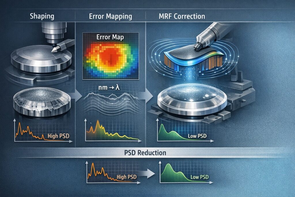
4. Erasing the Machine’s Memory: PSD and Spatial Frequencies
In the preceding chapters, we established the critical role of air-bearing spindles and the management of Non-Repetitive Run-out (NRR). However, even a state-of-the-art grinding process leaves a signature on the lens surface. This signature is not a random error; it is a collection of periodic ripples known as Mid-Spatial Frequency (MSF) errors. These ripples are effectively the “mechanical memory” of the machine—a record of every spindle vibration, every ball-screw oscillation, and every tool-path discretization step. In the world of high-end optics, these memories are the enemy of performance.
The Ghost in the Lens: Power Spectral Density (PSD)
To understand the impact of MSF errors, we must look beyond average roughness (Ra) and analyze the Power Spectral Density (PSD) of the surface. PSD represents the amplitude of errors as a function of their spatial frequency. Grinding typically leaves “spikes” in the PSD map—sharp peaks at specific frequencies corresponding to the spindle’s RPM or the feed rate of the axes. When light passes through a lens with these periodic ripples, it undergoes diffraction, creating “ghost images” and “flare” that reduce the system’s Modulation Transfer Function (MTF). A lens can be perfectly transparent and have a low Ra, yet still fail if its PSD spikes are too high.
MRF as a Physical Low-Pass Filter
Traditional polishing often struggles with MSF errors; rigid laps tend to “bridge” over the ripples, while soft pads may smear them into larger form errors. Magnetorheological Finishing (MRF) provides a unique solution because its removal mechanism is shear-mode dominant rather than impact-mode. The fluid ribbon acts as a physical low-pass filter. Because the MR fluid conforms to the surface at a molecular level but is controlled by a stable, averaged magnetic field, it selectively erases the high and mid-frequency ripples without introducing new ones.
Furthermore, MRF does not rely on mechanical bearings at the point of contact. The “tool” is a fluid ribbon supported by a magnetic field. This absence of a direct mechanical link means that the MRF process does not have its own ball-pass frequencies or mechanical harmonics to engrave into the glass. By removing the periodic noise left by the grinding stage, MRF restores the lens to its intended mathematical purity.
Selective Smoothing vs. Global Correction
One of the most powerful features of MRF is the ability to adjust the spatial resolution of the correction. By changing the size of the Tool Influence Function (TIF) through fluid chemistry or ribbon geometry, engineers can target specific frequency bands in the PSD map. If the metrology shows a dominant ripple at a 2mm period, a small TIF can be used to “de-ripple” the surface deterministically. This level of selective frequency control is what allows for the production of optics for EUV Lithography, where any spatial noise could ruin the diffraction-limited performance of the system.
The Frequency Axiom: “MRF does not introduce spatial frequency; it selectively removes it. While the spindle defines the shape, the MR fluid ribbon defines the purity of the light path by erasing the mechanical memories of the machine.”
5. The Chain of Command: Grinding-to-MRF Synergy
One of the most critical operational errors in ultra-precision manufacturing is treating Magnetorheological Finishing (MRF) as an isolated correction tool. In reality, MRF is the final link in a highly sensitive Process Chain. The success of the deterministic polishing stage is mathematically and physically “locked” by the quality of the preceding grinding stage. If the grinding spindle’s stability or the machine’s thermal management fails, the resulting errors may exceed the Capture Range of the MRF process, leading to a “Convergence Failure” where the lens can never reach its target specification.
The Capture Range and Form Prerequisite
The “Capture Range” refers to the maximum form error that a deterministic polishing process can effectively correct within a reasonable timeframe. While MRF is powerful, its removal rate is intentionally low to maintain nanometric control. If a ground lens enters the MRF stage with a form error exceeding 1-2 μm, the polishing time required to “level” the surface increases exponentially. This extended cycle time introduces new risks, such as fluid evaporation or thermal drift in the machine’s axes. Therefore, the grinding stage must act as the Primary Shaper, delivering a geometry that is already 99% accurate, allowing MRF to focus solely on the final 1% of “Wavefront Perfection.”
SSD: The Invisible Boundary
As discussed in our earlier deep-dive into aspheric grinding, Sub-Surface Damage (SSD) is the invisible enemy. If the grinding spindle exhibited high NRR or if the wheel was not perfectly trued, micro-cracks may extend tens of microns into the glass. MRF removes material atom-by-atom via shear stress. If the SSD layer is deeper than the intended MRF removal depth, those micro-cracks will remain. During the final polishing pass, these cracks can “bloom” or cause localized removal rate variations, resulting in mid-spatial frequency “scars” that destroy the PSD (Power Spectral Density) requirements. The “Chain of Command” dictates that grinding must limit SSD so that MRF can erase it completely.
The Synergy of Determinism
True synergy is achieved when the metrology data from the grinding stage is used to pre-calculate the MRF dwell-time map. By treating the grinding and polishing as a unified Digital Twin, engineers can adjust the grinding parameters to leave a specific “error signature” that is easiest for the MRF TIF (Tool Influence Function) to remove. This holistic approach reduces the total manufacturing time by 40-60% and is the primary reason why companies mastering both stages dominate the semiconductor and aerospace optics markets.
The Synergy Axiom: “MRF is a finisher, not a magician. The quality of the optical wavefront is born in the grinding spindle and only perfected in the MRF fluid. A failure in the first is uncorrectable in the second.”
6. Environmental Limits: The 1 mK Stability Barrier
As we descend into the nanometric realm of λ/20 and λ/40 wavefront accuracy, the distinction between the machine tool and its environment effectively disappears. In this regime, the Thermal Expansion Coefficient of the machine’s structural materials becomes the dominant source of error. For a standard 1-meter steel structure, a temperature change of just 0.01°C results in a linear expansion of 120 nm—an error that is five times larger than the entire tolerance budget for a high-end aspheric lens. This is the 1 mK Stability Barrier, where the air in the room must be treated as a critical machine component.
Micro-Thermal Gradients and TIF Drift
In Magnetorheological Finishing (MRF), the stability of the Tool Influence Function (TIF) is paramount. However, the MR fluid itself is a source of heat due to the energy dissipation from the high-pressure pumping system and the frictional shear at the polishing ribbon. If this heat is not managed through a refrigerated chiller controlled to within ±0.005°C, the fluid’s viscosity will drift. A drift in viscosity changes the “hardness” of the ribbon, which in turn alters the material removal rate. When this happens, the Dwell-Time Algorithm (which assumes a constant TIF) becomes invalid, and the process begins to “polish in” errors rather than correcting them.
Seismic Noise: The Floor as a Speaker
Beyond thermal stability, Seismic Isolation is the second pillar of the environmental limit. High-frequency vibrations from the factory floor—caused by nearby forklifts, HVAC units, or even external traffic—act as “acoustic noise” that modulates the gap between the fluid ribbon and the lens. In a deterministic process, this random modulation introduces Mid-Spatial Frequency (MSF) errors that the deconvolution algorithm cannot predict. To counter this, ultra-precision MRF systems must be mounted on active pneumatic isolation platforms that filter out vibrations down to the 0.5 Hz range, effectively “silencing” the floor.
Metrology Loop Uncertainty
The most insidious environmental trap is the Metrology-Machining Gap. If a lens is measured in a metrology room at 20.01°C and then polished in an MRF chamber at 20.05°C, the “apparent” form of the lens will have changed due to thermal expansion. The machine will then execute a correction for an error state that no longer exists in that environment. This is why high-end facilities utilize In-situ Metrology or “Integrated Metrology Loops,” where the measurement and the polishing occur in the same air-volume to ensure that the thermal state of the glass remains constant between the “Read” and “Write” cycles.
The Environmental Axiom: “In ultra-precision optics, the room is the machine. If you cannot control the temperature to the millikelvin, your deconvolution algorithm is simply a high-speed calculator for the wrong problem.”
7. Industrial Realities: Where Nanometers Turn Into Profit
Ultra-precision Magnetorheological Finishing (MRF) is not merely an academic exercise in fluid dynamics; it is the fundamental enabler of the multi-trillion-dollar digital and aerospace economy. By mastering the “Force-Stiffness-Math” trinity, industries have transitioned from mass production to “Mass Precision.” The ability to consistently produce surfaces with λ/20 accuracy has moved from being a laboratory miracle to an industrial requirement. In this final chapter, we examine the specific sectors where nanometric control translates directly into market dominance.
Semiconductor Lithography (EUV): The Picometric Frontier
The most demanding application of deterministic polishing is Extreme Ultraviolet (EUV) Lithography. The mirrors used in ASML systems must guide light at a wavelength of 13.5 nm. To achieve this without catastrophic scattering, the mirror surfaces must be finished to a form accuracy measured in picometers. MRF is the primary tool used to correct the multi-layer substrates of these mirrors. Without the ability to erase the spatial frequency errors left by the grinding spindles, the global transition to 3nm and 2nm semiconductor nodes would be physically impossible. In this sector, the MRF process is the “gatekeeper” of Moore’s Law.
Consumer Electronics: The AR/VR Immersion Gap
In the consumer market, particularly for Augmented and Virtual Reality (AR/VR), the challenge is weight versus fidelity. To make headsets wearable for long periods, lenses must be thin, lightweight aspheres. However, the human eye is incredibly sensitive to mid-spatial frequency errors (the “Ghosting” effect). By utilizing high-volume MRF lines, manufacturers can “de-ripple” aspheric molds and lenses at scale. This ensures that the Modulation Transfer Function (MTF) remains high across the entire field of view, eliminating the nausea and visual artifacts that plagued earlier generations of VR hardware.
Aerospace and Defense: IR Vision Systems
Infrared (IR) optics for missile seekers and satellite cameras often utilize hard, brittle materials like Silicon (Si) or Germanium (Ge). As we explored in Chapter 2, these materials are prone to fracture. MRF’s shear-mode removal allows for the final correction of these optics without the risk of propagating sub-surface damage. This leads to cameras that can “see” through thermal noise with unprecedented clarity, providing a strategic advantage in reconnaissance and high-altitude surveillance where every photon counts.
The Industrial Axiom:
“Precision is the ultimate competitive moat. In the nanometer economy, MRF did not just replace grinding; it replaced hope with calculation. Performance is no longer a goal — it is a deterministic result.”
References & Internal Technical Resources
Primary Engineering References
- • Golini, D., et al. (1999). Magnetorheological Finishing (MRF) for High-Precision Optics. Optical Manufacturing and Testing III.
- • Rowe, W. B. (2014). Principles of Modern Grinding Technology. Academic Press. (Analysis of SSD and the Grinding-Polishing interface).
- • Kordonski, W., & Shorey, A. B. (2007). Magnetorheological Polishing: A Review. International Journal of Modern Physics B.
- • Altintas, Y. (2012). Manufacturing Automation: Metal Cutting Mechanics, Machine Tool Vibrations, and CNC Design. Cambridge University Press.
Internal Technical Deep-Dive
To fully master the deterministic transition from grinding to atomic-level finishing, explore these specialized modules: