Aspheric Metrology Revisited: Why Modern Optics Measure Wavefronts, Not Shapes

1. The Measurement Paradox: Why Aspheres Defy Traditional Coordinates

In the history of precision engineering, measurement has always been the prerequisite for manufacturing. You cannot create what you cannot verify. However, as optics transitioned from simple spherical curves to complex aspheric and freeform geometries, the industry encountered a Fundamental Measurement Paradox. In a spherical system, every point on the surface is defined by a single radius originating from a unique center of curvature. This geometric symmetry allows for a stable, self-referencing coordinate system. An asphere, by definition, breaks this symmetry. It possesses no single center of curvature, meaning that every nanometer across its radial profile exists in a state of “geometric isolation.”

The Vanishing Reference Point

The primary challenge in aspheric metrology is the loss of a physical reference. When measuring a sphere, any misalignment in the measurement setup typically manifests as a simple “tilt” or “power” error that is easily subtracted. In aspheric metrology, however, a slight misalignment—known as Abbe Error or decenter—is mathematically “convolved” with the aspheric coefficients. This creates an induced coma or astigmatism in the measurement data that is indistinguishable from an actual manufacturing error. This leads to the first pillar of the paradox: To measure an asphere correctly, you must already know its exact position in 3D space with a precision that often exceeds the capability of the mechanical stage holding it.

Mechanical Shape vs. Optical Wavefront

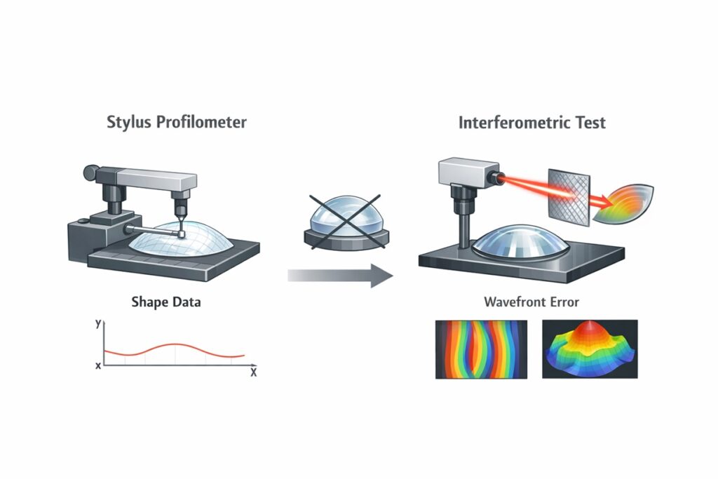
For decades, the standard response to this challenge was to use high-precision contact profilometry. Mechanical stylus instruments would trace the physical coordinates of the surface, providing a “Form Map.” But as we pushed into the λ/10 and λ/20 regimes, a conceptual chasm opened between “Shape” and “Performance.” A surface can be mechanically “correct” according to a stylus trace, yet fail spectacularly in an optical system. This is because mechanical measurements often lack the sensitivity to capture Mid-Spatial Frequency (MSF) errors—the microscopic ripples that do not change the macro-shape but do destroy the Optical Wavefront.

We must therefore acknowledge that in modern high-end optics, the physical shape of the lens is merely a proxy for the behavior of the light that passes through it. The “Measurement Paradox” forces us to stop asking “Is this point at the right X, Y, Z coordinate?” and start asking “How does this surface transform the incoming wavefront?” This shift from Coordinate-Based Metrology to Wavefront-Based Metrology is the defining revolution of the current era. It is the reason why we no longer “measure” aspheres in the traditional sense; we “solve” them through interference.

2. The Era of Physical Contact: Stylus and Mechanical Certainty

Before the widespread adoption of laser interferometry, aspheric manufacturing relied almost exclusively on Contact Profilometry. These instruments utilize a high-precision diamond stylus that physically traces the radial profile of the lens. The appeal of this method was its “Mechanical Certainty”—it provided a direct, traceable coordinate map in the X-Z plane. In the early days of CNC aspheric grinding, this 2D profile was the primary feedback loop used to calculate machine tool compensations. However, as optical requirements tightened, the inherent physical limitations of the stylus became a bottleneck for progress.

The Filtering Effect of Tip Radius

The most significant limitation of contact measurement is the Stylus Tip Radius. A stylus is not a mathematical point; it typically has a radius ranging from 0.5 μm to 25 μm. As the stylus moves across the surface, it acts as a Mechanical Low-Pass Filter. If the surface contains Mid-Spatial Frequency (MSF) ripples with a period smaller than the tip geometry, the stylus will “bridge” over the valleys, providing a smoothed version of reality. This creates a dangerous illusion of a high-quality surface when, in fact, the lens harbors high-frequency noise that will degrade the optical contrast.

Contact Pressure and Surface Integrity

Measurement itself is an act of physical interaction. To ensure the stylus remains in contact with the asphere during high-speed scanning, a specific Contact Force (often measured in millinewtons) must be applied. On soft optical materials or thin coatings, this pressure can cause local elastic or even plastic deformation. At the nanometer scale, the act of “measuring” can inadvertently “modify” the surface. Furthermore, the stylus is prone to “skipping” or “flying” if the scanning speed is too high or the aspheric slope is too steep, leading to data dropouts and false form readings that can mislead a deterministic grinding algorithm.

The 2D Profile vs. 3D Reality

Perhaps the most critical failure of traditional contact measurement is its Dimensional Limitation. A stylus trace provides a 2D cross-section of a 3D aspheric surface. It assumes that the lens is perfectly symmetrical around its optical axis. However, as we discussed in our spindle dynamics chapter, errors like Non-Repetitive Run-out (NRR) create non-rotationally symmetric errors (astigmatism, trifoil). A 2D trace is blind to these azimuthal variations. An engineer might see a perfect 2D profile and yet be baffled when the lens fails a 3D wavefront test. This “blindness” is what necessitated the transition to sub-aperture and full-field interferometry.

3. The Logical Collapse: When the “Master” Disappears

For centuries, the gold standard of precision was the Master Reference. To measure a meter, one compared a stick to the master meter in Paris; to measure a spherical lens, one used a “Master Glass” and observed the interference fringes (Newton’s Rings) between the two. This worked because a sphere is a unique geometric entity where any section of the curve matches every other section. But when the optical industry moved toward high-order aspheres, this entire logical foundation collapsed. We entered a regime where the measurement reference—the “Master Asphere”—simply ceased to exist in a physical form.

The “Chicken and Egg” Problem of Aspheric Masters

The fundamental requirement for any measurement is that the Reference must be significantly more accurate than the Object being measured. In spherical optics, creating a master sphere is relatively straightforward due to the self-correcting nature of the grinding process. However, to create a physical “Master Asphere,” one would need an existing metrology system capable of verifying it. But that metrology system would, in turn, need a master to calibrate it. This creates a circular dependency—a metrological infinite regress. In short: we cannot build a master asphere more accurate than our ability to measure it, and we cannot measure it without a master.

The Distortion of the “Null” Condition

In classical interferometry, the “Null Test” is the holy grail. It occurs when the incoming wavefront perfectly matches the surface shape, resulting in a “null” fringe pattern (a single solid color). With aspheres, a standard spherical wavefront hitting the surface creates a massive density of interference fringes—so dense that they become a blur, making it impossible to resolve the underlying nanometric errors. To achieve a “Null” condition for an asphere, you need a Null Compensator (a lens or mirror that distorts the light into an aspheric shape). But here is the trap: the compensator itself is an asphere with its own manufacturing errors. Any flaw in the compensator is “baked into” the measurement of the lens, leading to the False Positive error—a lens that looks perfect but fails because the reference was wrong.

The Shift to Mathematical Truth

The “Logical Collapse” of physical masters forced the industry to realize that the only stable reference for an asphere is Mathematics. We had to move from comparing “Glass to Glass” to comparing “Glass to Equation.” This realization paved the way for the Digital Revolution in metrology. We no longer look for a physical object that matches our lens; we create a Mathematical Wavefront that exists only in a computer’s memory or is encoded into a holographic plate. This shift represents the most profound change in optical history: we have traded the certainty of the physical master for the infinite precision of the digital algorithm.

4. The Mathematical Embodiment: CGH and the Null Test

As we established in the previous chapter, the physical “Master Asphere” is a logical impossibility at the λ/20 frontier. To break the cycle of metrological regress, we must transition from physical templates to Diffractive References. This is the role of the Computer Generated Hologram (CGH). The CGH is not a lens or a mirror in the traditional sense; it is a microscopic, lithographically etched diffraction grating that serves as the Physical Embodiment of a Mathematical Equation.

The Mechanics of Wavefront Transformation

In a standard interferometer, the laser produces a perfect spherical or planar wavefront. When this light hits a complex asphere, it reflects back as a “distorted” wave that the interferometer cannot interpret because the fringe density is too high. A CGH acts as a Wavefront Compensator. By calculating the exact phase shift required to neutralize the aspheric departure, we etch millions of concentric rings (diffraction zones) onto a quartz substrate. When the laser passes through the CGH, the diffracted light is reshaped into an aspheric wavefront that perfectly matches the ideal design of the lens.

The “Null” Philosophy: Subtracting Perfection

The power of the CGH lies in the Null Test. If the manufactured asphere is perfect, the wavefront reflected from the lens and the wavefront generated by the CGH will cancel each other out perfectly, resulting in a “Null” fringe (a zero-frequency pattern). Any fringe that appears in the interferometer is not the shape of the lens itself, but the Deviation from the Equation. This is a critical distinction: we are no longer measuring a surface; we are measuring the error of the surface. This allows us to focus the entire dynamic range of our sensors on the nanometric flaws, ignoring the macro-geometry that is already accounted for by the CGH.

Traceability and Lithographic Precision

Why is a CGH more reliable than a physical master? The answer lies in Lithographic Traceability. The patterns on a CGH are created using the same electron-beam (E-beam) lithography tools used to make microchips. The placement accuracy of these diffraction zones is controlled to within a few nanometers across the entire substrate. Because the “Reference” is defined by the position of these lines—which is a function of the machine’s laser-interferometer-controlled stage—the optical truth of the CGH is directly traceable to the international standard for length (the meter).

5. Beyond the Null: Stitching and Slope-based Metrology

While the CGH-based null test is the gold standard for high-precision aspheres, it faces practical limitations when dealing with extreme apertures or highly complex freeform geometries. A single CGH may not be able to “null” a surface with severe departures, or the cost of producing a massive CGH for a meter-class mirror may be prohibitive. To overcome these barriers, the industry has developed Non-Null Metrology techniques that rely on sophisticated mathematical reconstruction: Sub-aperture Stitching and Deflectometry.

Sub-aperture Stitching Interferometry (SSI)

Sub-aperture Stitching Interferometry (SSI) is a “divide and conquer” approach. Instead of attempting to measure the entire asphere at once, the system takes multiple high-resolution interferometric “snapshots” of small, localized regions (sub-apertures). Each sub-aperture is measured at its own local “best-fit” sphere, where the fringe density is manageable. The challenge lies in the Stitching Algorithm: the software must mathematically align these overlapping patches into a single, seamless 3D map. This requires a picometric understanding of the machine’s mechanical axes to compensate for the “piston” and “tilt” errors introduced as the lens moves between positions.

Deflectometry: Measuring the Slope of Light

Interferometry measures the Phase of light, which is directly proportional to the surface height. Deflectometry, on the other hand, measures the Slope (the first derivative of the height). By reflecting a known pattern (like a checkerboard or sinusoidal fringe) off the asphere and observing how the pattern deforms, we can calculate the local surface normal at every point. Deflectometry is exceptionally powerful for Freeform Metrology because it does not require a null reference. It can measure surfaces with massive departures that would “blind” a standard interferometer. However, because it is a slope-based measurement, it is highly sensitive to Mid-Spatial Frequency (MSF) noise, making it an ideal companion to MRF processes that target PSD correction.

Frequency-Domain Mapping

The choice between Stitching and Deflectometry often comes down to the Spatial Frequency of the errors being targeted. Stitching provides absolute form accuracy for low-frequency errors (the global shape), while Deflectometry provides high-fidelity data on the mid-frequency ripples (MSF). In advanced aspheric manufacturing, these two data sets are often “fused” together to create a multi-scale surface map. This holistic view is what allows the deterministic polishing cycle to address everything from the 100 mm form to the 1 mm periodic ripples left by the grinding spindle.

6. The Integrated Loop: In-situ Metrology and Digital Twins

In the traditional optical shop, metrology and manufacturing exist in two different worlds. A lens is ground, removed from the machine, transported to a climate-controlled metrology lab, measured, and then brought back for polishing. At the micron level, this works. At the nanometer level, this separation is a recipe for failure. The moment a lens is removed from its fixture and its environment changes by even a fraction of a degree, the “Physical Context” of the measurement is lost. This is the final barrier to deterministic manufacturing: the metrology gap.

Thermal Memory and the Metrology Gap

As discussed in our chapter on thermal stability, a 1 mK temperature difference can cause a 120 nm expansion in a meter of steel. If the metrology room is at 20.00°C and the MRF machine is at 20.05°C, the lens “shifts” its shape between the two environments. The measurement taken in the lab becomes a “False Map” for the machine. Furthermore, the act of re-fixturing the lens introduces centering and tilt errors that are nearly impossible to eliminate manually. For the deconvolution algorithm to work with 95% convergence, the machine must “see” the lens exactly as it “holds” it.

In-situ Metrology: Closing the Loop

In-situ Metrology solves this by integrating the measurement system (often a probe or a sub-aperture interferometer) directly into the machining center. The lens never leaves its chuck. This allows for a Closed-Loop Manufacture where the machine measures the surface, calculates the dwell-time map, polishes for a cycle, and immediately re-measures to verify the result. By keeping the lens in a constant thermal and mechanical state, we eliminate the variables of re-fixturing and environmental drift. This is the physical foundation of the Digital Twin: the software model of the lens and the physical lens on the spindle are always in perfect synchronization.

The Data-Driven Process Chain

In this integrated loop, the metrology data is no longer just a “Quality Report”—it is the Primary Control Input. The feedback loop allows the system to compensate for TIF (Tool Influence Function) drift in real-time. If the in-situ measurement shows that material removal is 2% slower than predicted (perhaps due to fluid aging), the Digital Twin automatically adjusts the dwell-time for the next pass. This level of self-correction is what enables the production of aspheres for EUV Lithography and Satellite Optics, where the cost of a single “wrong” polishing pass can be hundreds of thousands of dollars.

7. Conclusion: The New Standard of Perception

The journey from the diamond stylus to the Computer Generated Hologram represents more than just a technological upgrade; it is a fundamental shift in how humanity perceives precision. We have moved from the Mechanical Era, where truth was found in the physical contact of a probe, to the Wavefront Era, where truth is found in the interference of light. This transition was not a choice, but a physical necessity dictated by the nanometric requirements of the 21st century.

The End of the “Shape” Era

For decades, the engineering goal was to produce a lens that matched a CAD model’s XYZ coordinates. Today, we realize that a “perfect” XYZ shape can still fail due to mid-spatial frequency ripples, subsurface damage, or material inhomogeneities. As we have seen through this series, Aspheric Metrology has evolved to become the “filter” that separates mechanical noise from optical signal. We no longer ask if the glass is in the right place; we ask if the light wave it produces is in the right phase.

The Convergence of Manufacturing and Metrology

The ultimate takeaway for the modern manufacturing engineer is the Collapse of the Process Boundary. In the world of λ/40 optics, metrology is not the “last step”—it is the continuous heartbeat of the machine. The integration of CGH references, stitching algorithms, and in-situ feedback loops has created a deterministic manufacturing environment where performance is no longer an expected outcome, but a calculated certainty.

References & Internal Technical Resources